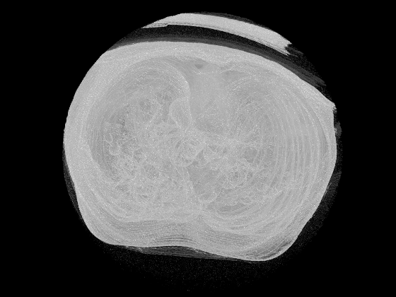
Rapid 3D Medical Imaging Reconstruction

Caption: Reconstructed 3D medical image.

Idea and Introduction: Currently a lot of 3-D medical imaging reconstruction takes a lot of computational power and tends to only provide a “pretty picture” and does not provide any additional information for diagnostics (source). Since edges often highlight the details of images, an edge based approach to medical imaging reconstruction hopes to increase the diagnostic potential of 3D medical images, and to reduce computational needs for 3D image reconstruction. Note that medical images are often conducted in 2D slices that move through a volumetric portion of a patient (Thus 3D views can be made from these 2D slices).

Summary: I devised an image processing algorithm utilizing edge detection, median filtering, unsharp masking, and histogram normalization that preprocessed the images for 3D image construction. The 3D image reconstruction was conducted using the volshow() function in MATLAB utilizing a maximum intensity projection. Using a sample lung CT phantom, I tested my processing. Although there are several improvements that are needed to be made, this project demonstrated that rapid 3D medical imaging is possible.

The code written for this project is on my github.

Developing The Edge Detection Process

The fundamental step for this approach of 3D image reconstruction, is to run a medical image through an edge detection algorithm. However, it is not ideal to solely use edge detection on a medical image; as an image will contain noise and edges that are not “easy” to detect. The goal here is to both increase the true positive rate while decrease the false positive rate for an edge. Therefore both a low pass filter (noise reduction) and a high pass filter (sharpening) is ran on the image along with a edge detection algorithm.

The noise reduction method that is used is simply median filtering as it easily reduces noise by applying a median intensity over a selected slice of an image. This noise reduction method is used as it is not computationally heavy.

The sharpening method that is used is unsharp masking as this is a commonly used method to sharpen an image.

Another aspect to consider for the overall image processing algorithm is the edge detection algorithm to use. There are four overall edge detection algorithms: Sobel, Prewitt, Laplacian, and Canny.

I decided to use the Sobel operator as this edge detection model has a short computation time. The Sobel operation involves just convoluting a gradient over the image, and is a relatively accurate edge detection algorithm. While the algorithm may be sensitive to noise, but since the image undergoes noise reduction (through a median filter), noise is not necessarily a issue.

The next step is to decide what order of steps the overall algorithm should undertake. There are six possible orders the image could undergo:

• Noise Reduction –> Sharpening –> Edge Detection Image (Image 1 in figure below)
• Noise Reduction –> Edge Detection –> Sharpening Image (Image 2)
• Sharpening –> Noise Reduction –> Edge Detection Image (Image 3)
• Sharpening –> Edge Detection –> Noise Reduction Image (Image 4)
• Edge Detection –> Noise Reduction –> Sharpening Image (Image 5)
• Edge Detection –> Sharpening –> Noise Reduction (Image 6)

The following image shows those following processes, with the following order:

• Row 1 order: Image 1, Image 2, Image 3
• Row 2 order: Image 4, Image 5, Image 6

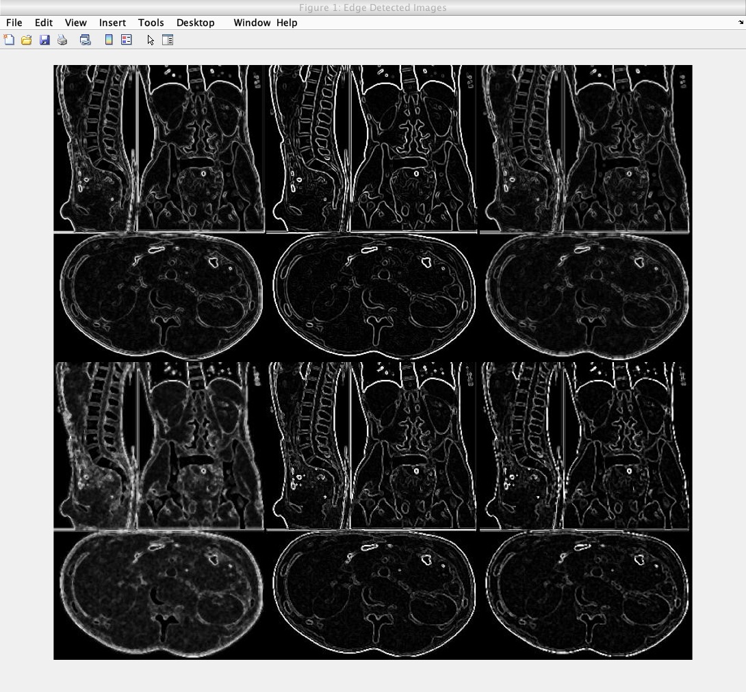
Caption: A test of all six edge detection models outlined above.

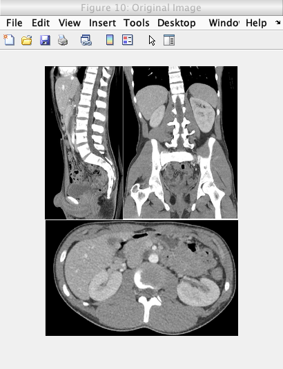
The above processes were ran on this image:

Caption: The original image undergoing edge detection.

The second image on the first row shows that undergoing noise reduction first then edge detection then sharpening provides the ideal edge detected image. This image also has the highest resolution and the highest amount of correct edges; reducing the edge detection false negative rate, while increasing the true positive rate.

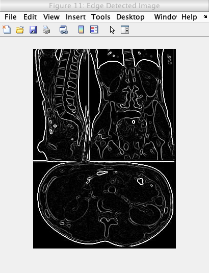
This is the image showing an image solely undergoing the Sobel edge detection model:

Caption: The original image undergoing edge detection solely through the Sobel operator.

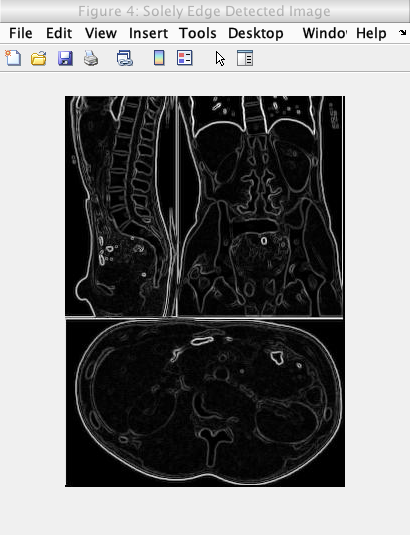
While this is the image showing the image undergoing the process of noise reduction, edge detection, and sharpening:

Caption: The original image undergoing edge detection undergoing noise reduction, edge detection, and sharpening.

Thus the process of undergoing noise reduction, edge detection, and sharpening in the order was found to be the ideal edge detection model.

3D Volume Generation Attempt

I initially thought that running my edge detection model on sample medical images to generate a 3D model would run succesfully. However that was not the case. The 3D volume was generated using a maximum intensity projection with the MATLAB volshow() function.

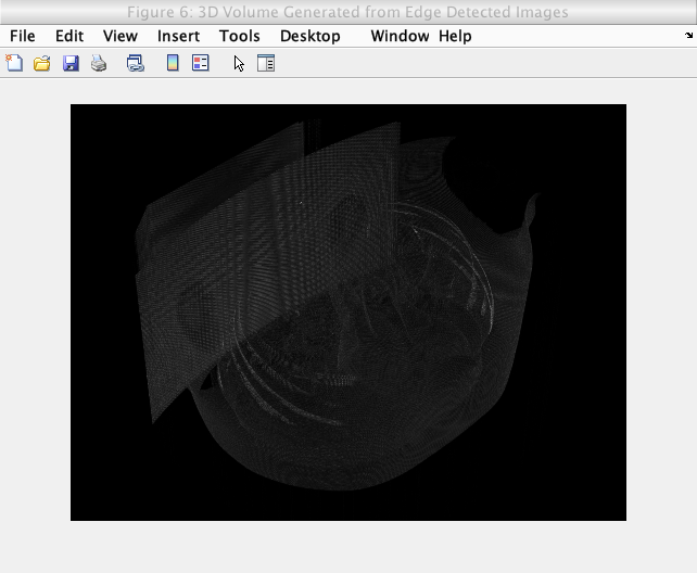
Caption: Initial 3D volume generation attempt.

As seen in the generated volume, no major details can be seen. This was due to the images not having enough information (edges are simply not enough for the volume generation).

Adapting the Image Processing Algorithm

My first attempt to counteract the issues above, was to simply overlay the edge detected images on the original image using a simple averaging of intensity values in the images. However, this averaging lowered the general intensity of the image which lowers the brightness and contrast of the image. The figure below shows the effect of this overlay and the lowered brightness and contrast.

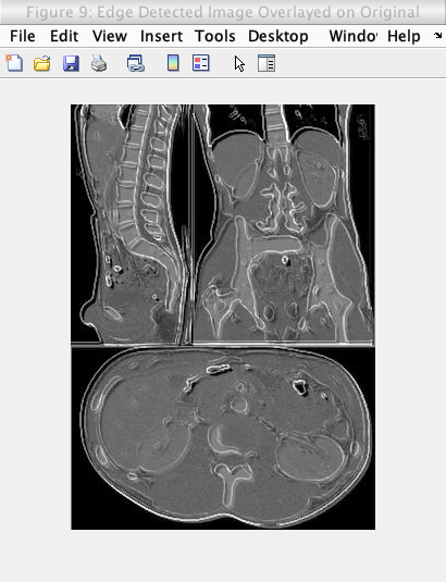
Caption: Edge detection (of the original image) overlayed on the original image using pixel-wise averaging.

After overlaying the edge detected image, a histogram equalization is conducted on the image. A histogram equalization in general involves equalizing the histogram of an image over a set intensity range (generally 0 to 255) to increase the contrast of an image. This increase is contrast is due to the fact that the equalization makes the image data as close to a normal distribution as possible.

This histogram equalization is also made to be adaptive by identifying the best equalization value that gives the best contrast.

The histogram equalization is done with the following steps:

• 1) Calculate the histogram (Probability Distribution Function) of the Image
• 2) Calculate the Cumulative Distribution Function of the image from the above Probability Distribution Function
• 3) Calculate the adaptive equalization value or use specified value Note: adaptive equalization process is outlined later
• 4) Apply equalization with the below function New pixel value = 1 + (equalization value * (cdf[index] - minimum of cdf)/ (number of pixels in image - minimum of cdf)

The identification of the best equalization value is conducted as following:

• 1) Loop through all possible intensities for normalization
• 2) Equalization data for each equalization value
• 3) Get histogram of that equalized data
• 4) Compare that histogram with an ideal histogram of normal distribution of intensities
• 5) Comparison is done by calculating a KL divergence for the normalization histogram and ideal histogram
• 6) The intensity value with the lowest KL divergence value is used as the equalization value

This intensity value indicates that the least amount of data would be lost if an image with the calculated histogram replaces an image with the histogram of the ideal histogram.

However after the adaptive equalization was conducted, it was found that the brightness of the image did not increase, so a “non-adaptive” equalization was conducted again with an equalization value of 216. This equalization value was used as it is about 85% of the maximum intensity of the image (so an image that is bright but not “too” bright was created). The figures below shows this equalization process.

As shown by the images below, the adaptive normalization was able to increase the contrast of the overlayed image, while the renormalization value was able to increase the brightness of the overlayed image while maintaining the increased contrast from the adaptive equalization.

Caption: Original image.

Caption: Edge detected image.

Caption: Edge detected image overlayed on original image.

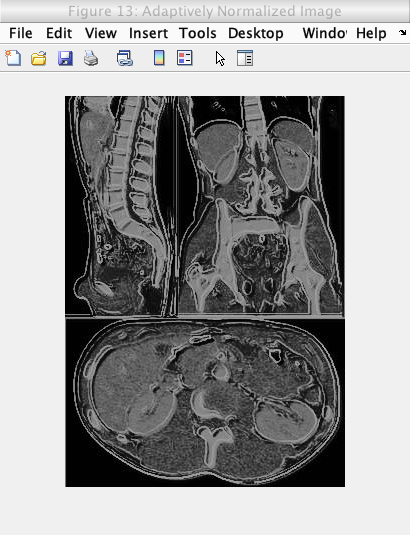
Caption: Adaptively normalization of above image.

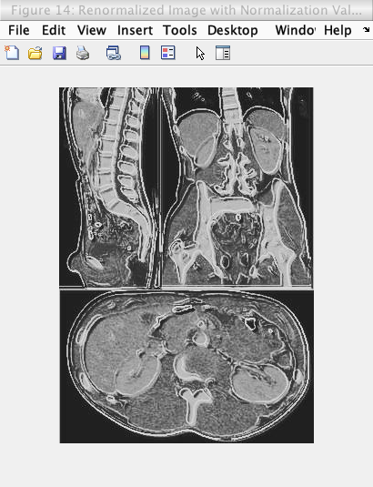
Caption: Renormalized image (to 85% maximum image intensity) of above image.

The 3D Volume Generation

The final step for the processing algorithm for the medical images was thresholding out the noise. Due to the process of the normalization on the images, the signal and noise components of the image are split, effectively allowing thresholding at an intensity value just below the maximum intensity of each processed image.

The following image shows the thresholding on a slice of a Lung phantom image.

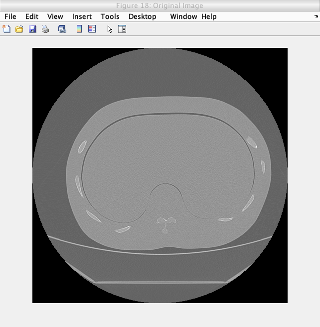
Caption: The original image.

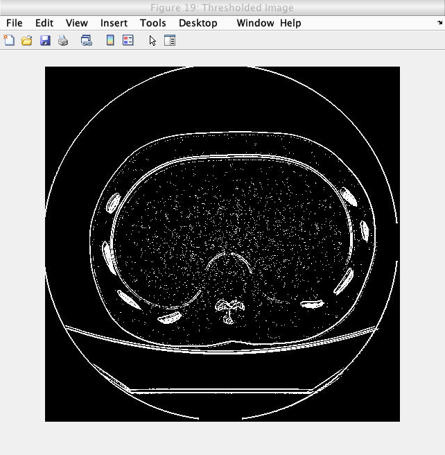
Caption: The thresholded image.

After completing the processing algorithm development. The following process was used to generate the 3D volume:

• 1) Read medical images
• 2) Convert medical images to uint8 RGB image format
• 3) Run all medical image slices through image processing algorithm
• 4) Use volshow() with maximum intensity projection function in MATLAB on processed images to generate 3D image

The following images shows the results of the volume generation for a lung phantom from the Cancer Imaging Archive(TCIA):

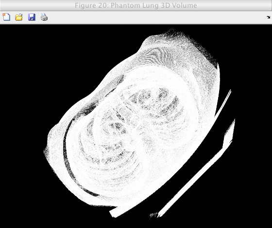
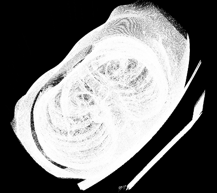
Caption: A view of the generated 3D volume.

Caption: A view of the generated 3D volume.

The following video shows the 3D volume being generated:

Caption: A video of the 3D volume generation.

And finally the video shows the viewing of the 3D volume:

Caption: A video of the 3D volume generation.

Conclusions, Future Improvements

Positives:

• 1) In general, regardless of image quality, the constructed volume is able to show most of the outer details of objects in the volume while highlighting some of the inner details of objects in the volume.
• 2) A relatively fast 3D image construction is able to be done.
• 3) The image processing algorithm increases contrast and brightness of a medical image while not degrading the medical image resolution and the processed images are successfully able to be used to generate 3D images of acceptable quality
• 4) A relatively large amount of noise is able to be removed from images (although some noise still appears in the volumes). It is important to note that a significant amount of noise is removed to the point that the noise does not construct false objects in the volumes
• 5) Pending enhancements to the computation time in the image processing algorithm, this 3D image reconstruction has potential to become a strong and fast way to construct 3D images from medical images
• 6) This algorithm can be easily modified to work for all imaging modalities (such as X-Ray CT, ultrasound, and MRI)
• 7) It appears that these volumes have potential to be used for diagnostic purposes especially is volume is adapted to have a certain range of slices used, and can have specific slices be shown alongside the original dicom image and processed dicom image if it is required

Negatives:

• 1) The use of the volshow() function leads to saturations of certain intensities in the volume which makes it hard to look at objects within the volume, however this can be counteracted by changing the camera angle of the volume
• 2) The volshow() function does not account for the slice thickness of the dicom images, which leads to a volume being smaller than its “real” size equivalent
• 3) Median filtering is used for noise-reduction which may not be the best way to filter out noise in the images
• 4) A single edge detection algorithm does not be needed to be used, multiple edge detection algorithms can be used in conjunction to increase the true positive rate
• 5) Unsharp masking is the process for sharpening which may not be the most ideal way to sharpen an image
• 6) Using an average of intensities value for the overlay of the edge detected image over the original image is not the best way to overlay the edge detected image over the original image
• 7) The equalization operation does accentuate a considerable amount of noise in the image (even though it is later thresholded out)
• 8) The adaptive equalization essentially loops through all the equalization amounts (0-255) to find the ideal contrast enhancing equalization, but it was observed that the adaptive equalization seems to occur in the equalization value range of 100-200. Several adaptive equalizations could be done on a wide set of medical images to give a strong estimate of the range of equalization amounts that could be looped through (this would reduce calculation time by at least 3 times)
• 9) There is no adaptive thresholding currently, this needs to be adjusted for the data set

Future Improvements:

• 1) A custom volshow() function should be built to construct a more ideal volume that can have objects that are more easy to view and this custom function could give the option to “peel off” layers in the z-direction to also increase viewability of the volume
• 2) Since a single slice is assumed to be one unit of a slice thickness slices can be replicated x amount of times to have each slice represent its unit magnitude of slice thickness
• 3) A Weiner filter can be used for noise reduction as this is a highly adaptive way to filter out noise
• 4) Multiple edge detection algorithms can be used in conjunction to increase the true positive rate (of an edge), and the sobel algorithm can be used in conjunction with more complex (yet iterative) edge detections (this includes the Canny edge detection algorithm)
• 5) A different and more adaptive and complex sharpening operation can be used instead of using unsharp masking to sharpen images. A process can also be developed to adaptively sharpen an image
• 6) A different method can be used to overlay the edge detected image over the original image, one potential method could be a median based overlay than a mean based overlay
• 7) As stated above: several adaptive equalizations could be done on a wide set of dicom images to give a strong estimate of the range of equalization amounts that could be looped through (this would greatly reduce calculation time)
• 8) A method to adaptively threshold the image can be generated or more simplistically a GUI can be created to have a technician to select the ideal threshold value for the set of medical images
• 9) Machine learning can be used for methods to adaptively apply a filter or algorithm on the medical images. This can be especially used for adaptive sharpening, adaptive equalization, and adaptive thresholding in the image processing algorithm
• 10) A machine learning based edge detection algorithm could also be used (this is most likely to increase the true positive rate of edges)